
A carbon dioxide graph can rise over decades while moving down during part of each year. Those two features are not contradictory. They describe changes occurring on different timescales within a system that exchanges carbon between the atmosphere, land and ocean.
The first step is to distinguish an amount stored from an amount moving. The second is to distinguish a seasonal pattern from the longer trend. A fictional bookkeeping exercise makes both distinctions visible without pretending to reproduce the complexity of the real Earth.
Stocks and flows answer different questions
A stock is the amount held in a reservoir at a particular time. A flow is a transfer over an interval. The atmosphere contains a stock of carbon; photosynthesis, respiration, ocean exchange and other processes move carbon between reservoirs.
NOAA’s carbon-cycle overview describes sources as processes that release carbon dioxide to the atmosphere and sinks as those that remove it. A place or process can participate in exchanges in both directions. What matters for a change in the atmospheric stock is the balance of the transfers.
An annual emission rate therefore cannot be read as though it were the atmospheric concentration. Nor can a large natural exchange be compared with an additional input without considering the corresponding removal. The units and the accounting boundary are part of the claim.
A box with counters
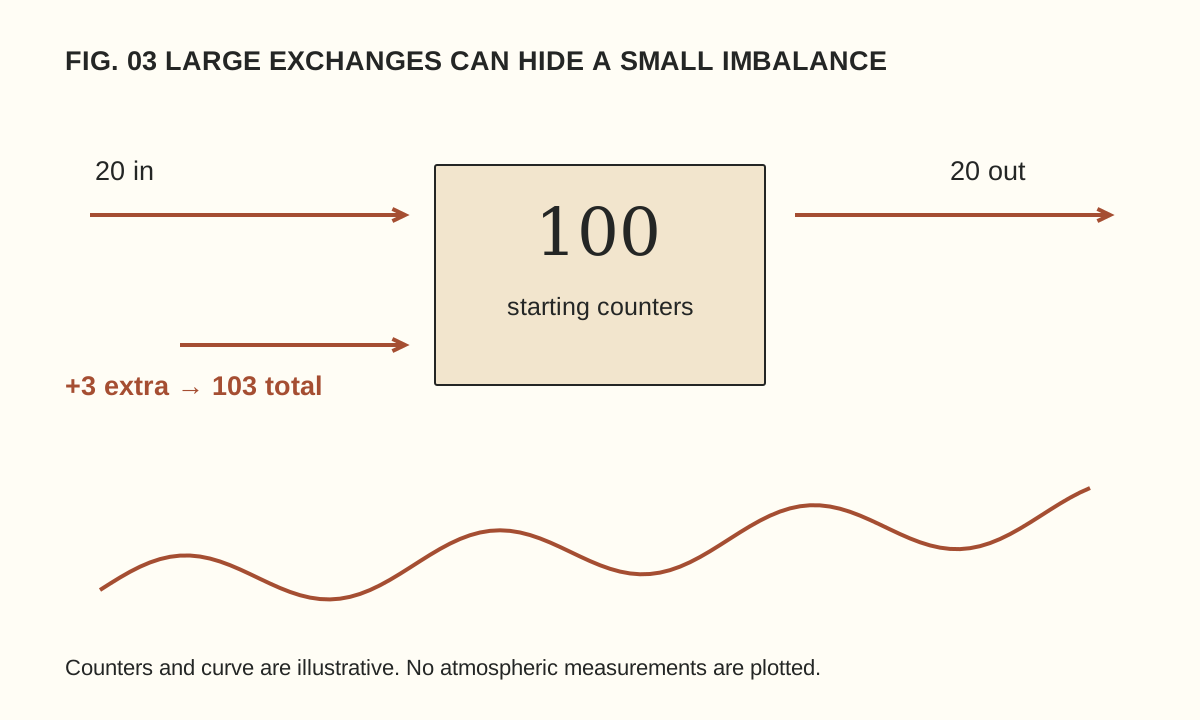
Imagine a box containing 100 counters. During one round, 20 counters enter and 20 leave. The box still contains 100. During the next round, the same exchanges occur but an extra three counters enter from another store. Unless removals also change, the box finishes with 103.
The extra three are smaller than the gross exchange of twenty in either direction, yet they change the total. This is an original arithmetic model, not an estimate of actual carbon flows. Its purpose is to show why comparing an added input only with a large natural input can miss the balancing output.
Now allow the outgoing flow to increase by one counter. The stock grows by two instead of three. A responding sink reduces the accumulation in this model, but does not erase it. If the outgoing flow eventually matched all incoming flows, the stock would stop growing at its new level; it would not automatically return to the old one.
Why the line moves with the seasons
NOAA’s greenhouse-gas network explanation connects the seasonal carbon dioxide cycle with the changing balance between photosynthesis and respiration. The northern hemisphere’s large land areas make that seasonal pattern particularly prominent in many records.
Think of a repeating wave placed on a gently rising ramp. During part of each wave, the line slopes downward; the ramp can still carry each year’s overall pattern higher. The drawing accompanying this article uses that idea schematically. It contains no observed concentrations and should not be mistaken for a monitoring record.
To compare like with like in a real seasonal series, examine corresponding months or use the provider’s documented trend product. Selecting a spring peak and an autumn low can reveal the seasonal cycle while saying little about the change from one year to the next.
Read the axes before the headline
A graph may show concentration, annual growth, emissions, a seasonal adjustment or an anomaly relative to a reference period. Each can be useful, but they answer different questions. Check the units, location, averaging period and treatment of missing observations.
Parts per million describes a proportion. A mass per year describes a flow. Tonnes of carbon and tonnes of carbon dioxide are also different quantities: carbon dioxide includes oxygen as well as carbon. A careful comparison keeps the same definition throughout rather than treating every carbon-related number as interchangeable.
NOAA publishes a global atmospheric carbon dioxide data page with its own methods and references. Read those explanations when using the data. A measurement from one station, a global estimate and a graphic designed for teaching are not equivalent products.
Fast and slow do not mean isolated
NASA’s carbon-cycle backgrounder describes exchanges through living systems alongside much slower geological pathways. Burning fossil fuels transfers carbon from long-stored material into the active atmosphere–land–ocean system. Land-use changes can also alter storage and exchange.
“Natural” and “human” are useful distinctions for particular processes, but the resulting carbon participates in a connected system. The ocean and ecosystems can respond to changed conditions. Those responses do not make the original addition disappear from the accounting question.
Our counter model cannot describe temperature feedbacks, ocean chemistry or regional differences. That limitation is deliberate. It teaches conservation and net change; it does not predict the future climate or provide a complete carbon budget. A model should be judged partly by whether it states the question it can answer.
Try a transparent reading exercise
- Choose one documented data series and write its name, unit and coverage period.
- Identify whether the line represents a stock, a flow or a derived trend.
- Mark two comparable dates without changing the averaging definition.
- Describe the observed change before proposing a cause.
- Read the source’s explanation of uncertainty, adjustment and coverage before drawing a wider conclusion.
If you make a teaching graph, label invented values as invented. If you use actual data, retain the source and the transformation steps. A smoothed line should not silently replace the original observations, and a dramatic axis choice should not substitute for an explanation of scale.
Keep the claim proportional to the evidence
A seasonal decline does not by itself demonstrate a reversal of a long-term increase. A rising concentration does not tell you the contribution of every individual source without further analysis. Both statements follow from asking what the graph actually measures.
For the same reason, numerical precision needs context. Our measurement guide explains why a result and its uncertainty belong together. Reading the carbon cycle becomes easier when the accounting is explicit: what is stored, what moves, over which interval and across which boundary?