
PNIS

Science, with the working shown

Look closer. Ask better questions.

Science is a way of asking questions, testing explanations and changing your mind when the evidence changes. These guides make the reasoning visible, with sources, examples and the limits of what we know.

Earth

The carbon cycle has stocks, flows and seasons. Here is how to read them.

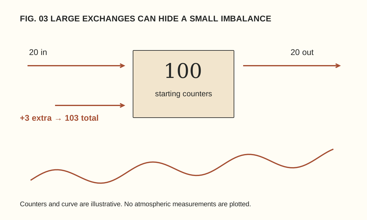
A box starts with 100 counters; 20 enter and 20 leave, then 3 extra raise the total to 103. A separate schematic wave rises over time. Not actual carbon data.

A carbon dioxide graph can rise over decades while moving down during part of each year. Those two features are not contradictory. They describe changes occurring on different timescales within a system that exchanges carbon between the atmosphere, land and ocean.

The first step is to distinguish an amount stored from an amount moving. The second is to distinguish a seasonal pattern from the longer trend. A fictional bookkeeping exercise makes both distinctions visible without pretending to reproduce the complexity of the real Earth.

Stocks and flows answer different questions

A stock is the amount held in a reservoir at a particular time. A flow is a transfer over an interval. The atmosphere contains a stock of carbon; photosynthesis, respiration, ocean exchange and other processes move carbon between reservoirs.

NOAA’s carbon-cycle overview describes sources as processes that release carbon dioxide to the atmosphere and sinks as those that remove it. A place or process can participate in exchanges in both directions. What matters for a change in the atmospheric stock is the balance of the transfers.

An annual emission rate therefore cannot be read as though it were the atmospheric concentration. Nor can a large natural exchange be compared with an additional input without considering the corresponding removal. The units and the accounting boundary are part of the claim.

A box with counters

Imagine a box containing 100 counters. During one round, 20 counters enter and 20 leave. The box still contains 100. During the next round, the same exchanges occur but an extra three counters enter from another store. Unless removals also change, the box finishes with 103.

The extra three are smaller than the gross exchange of twenty in either direction, yet they change the total. This is an original arithmetic model, not an estimate of actual carbon flows. Its purpose is to show why comparing an added input only with a large natural input can miss the balancing output.

Now allow the outgoing flow to increase by one counter. The stock grows by two instead of three. A responding sink reduces the accumulation in this model, but does not erase it. If the outgoing flow eventually matched all incoming flows, the stock would stop growing at its new level; it would not automatically return to the old one.

Why the line moves with the seasons

NOAA’s greenhouse-gas network explanation connects the seasonal carbon dioxide cycle with the changing balance between photosynthesis and respiration. The northern hemisphere’s large land areas make that seasonal pattern particularly prominent in many records.

Think of a repeating wave placed on a gently rising ramp. During part of each wave, the line slopes downward; the ramp can still carry each year’s overall pattern higher. The drawing accompanying this article uses that idea schematically. It contains no observed concentrations and should not be mistaken for a monitoring record.

To compare like with like in a real seasonal series, examine corresponding months or use the provider’s documented trend product. Selecting a spring peak and an autumn low can reveal the seasonal cycle while saying little about the change from one year to the next.

Read the axes before the headline

A graph may show concentration, annual growth, emissions, a seasonal adjustment or an anomaly relative to a reference period. Each can be useful, but they answer different questions. Check the units, location, averaging period and treatment of missing observations.

Parts per million describes a proportion. A mass per year describes a flow. Tonnes of carbon and tonnes of carbon dioxide are also different quantities: carbon dioxide includes oxygen as well as carbon. A careful comparison keeps the same definition throughout rather than treating every carbon-related number as interchangeable.

NOAA publishes a global atmospheric carbon dioxide data page with its own methods and references. Read those explanations when using the data. A measurement from one station, a global estimate and a graphic designed for teaching are not equivalent products.

Fast and slow do not mean isolated

NASA’s carbon-cycle backgrounder describes exchanges through living systems alongside much slower geological pathways. Burning fossil fuels transfers carbon from long-stored material into the active atmosphere–land–ocean system. Land-use changes can also alter storage and exchange.

“Natural” and “human” are useful distinctions for particular processes, but the resulting carbon participates in a connected system. The ocean and ecosystems can respond to changed conditions. Those responses do not make the original addition disappear from the accounting question.

Our counter model cannot describe temperature feedbacks, ocean chemistry or regional differences. That limitation is deliberate. It teaches conservation and net change; it does not predict the future climate or provide a complete carbon budget. A model should be judged partly by whether it states the question it can answer.

Try a transparent reading exercise

  1. Choose one documented data series and write its name, unit and coverage period.
  2. Identify whether the line represents a stock, a flow or a derived trend.
  3. Mark two comparable dates without changing the averaging definition.
  4. Describe the observed change before proposing a cause.
  5. Read the source’s explanation of uncertainty, adjustment and coverage before drawing a wider conclusion.

If you make a teaching graph, label invented values as invented. If you use actual data, retain the source and the transformation steps. A smoothed line should not silently replace the original observations, and a dramatic axis choice should not substitute for an explanation of scale.

Keep the claim proportional to the evidence

A seasonal decline does not by itself demonstrate a reversal of a long-term increase. A rising concentration does not tell you the contribution of every individual source without further analysis. Both statements follow from asking what the graph actually measures.

For the same reason, numerical precision needs context. Our measurement guide explains why a result and its uncertainty belong together. Reading the carbon cycle becomes easier when the accounting is explicit: what is stored, what moves, over which interval and across which boundary?
Methods

What the uncertainty beside a measurement is trying to tell you

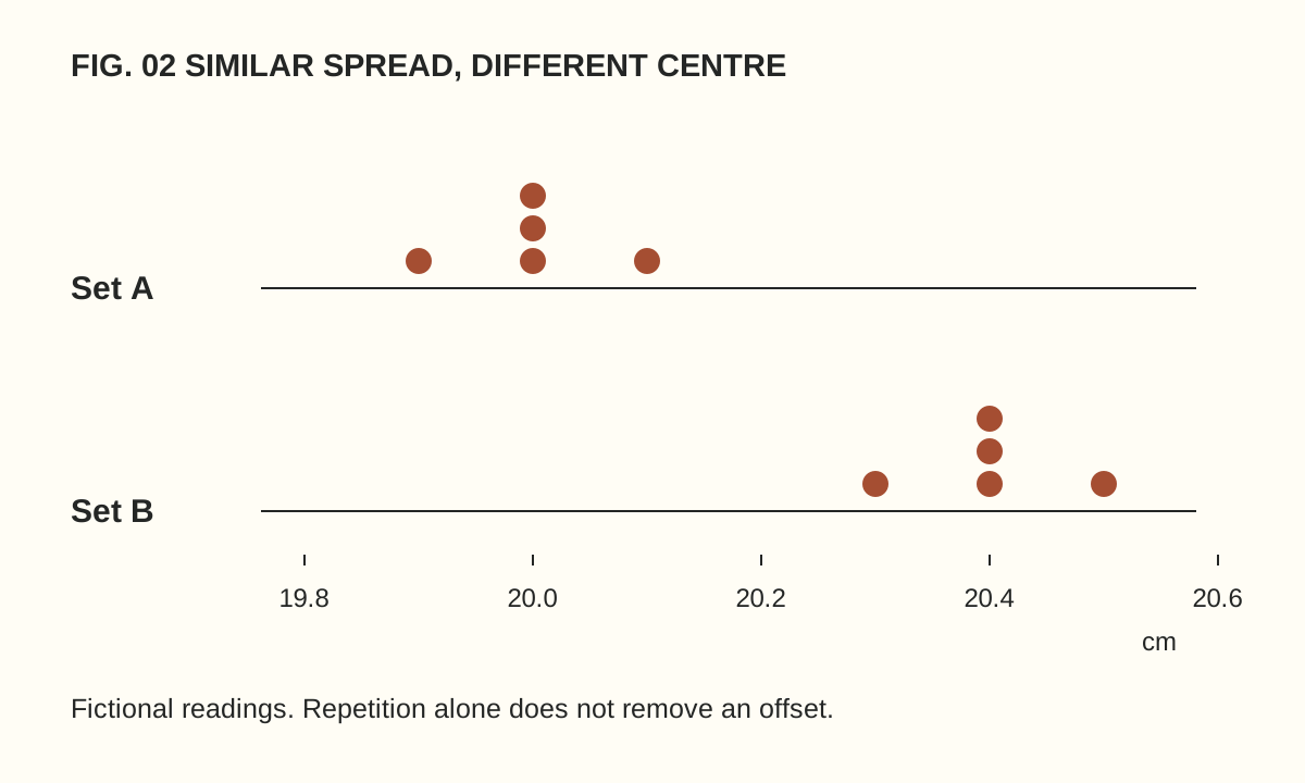
Dotplots of invented readings centred at 20.0 and 20.4 centimetres with similar spread illustrate that repeatability does not remove a systematic offset.

A result written as 20.03 looks more authoritative than one written as about 20. Yet extra digits do not explain the instrument, the procedure or the sources of variation. A measurement becomes informative when the number arrives with enough context to understand what it means.

Uncertainty is part of that context. It is not an apology attached to otherwise perfect science, nor a convenient way to dismiss a result. It describes the limits of the measurement under a stated set of information. A small classroom-style example makes the distinction concrete.

Decide what is being measured

Suppose we want the length of a rectangular card. Which edges define the length? Is the card lying flat? Are we measuring at the top, centre or bottom? A slightly irregular object can produce different results even when everyone uses the ruler correctly.

These questions define the quantity being measured. They are not pedantic additions after the “real” work. If two people measure different features, averaging their numbers does not repair the mismatch. A useful record begins with an operational description that another person could follow.

For our fictional exercise, let the task be the distance between two marked points on a card lying flat on a table. We use the same ruler and read it from directly above. Nothing here is a reported laboratory experiment; the numbers below are invented to illustrate the reasoning.

What repeated readings show

Imagine readings of 20.0, 20.1, 20.0, 19.9 and 20.0 centimetres. Their mean is 20.0 cm. The small spread tells us something about variation under this particular procedure. It does not establish that the ruler’s scale is correct or that the marked points represent the feature we intended to measure.

Now imagine a second set: 20.4, 20.5, 20.4, 20.3 and 20.4 cm. It has a similar spread but a different centre. If the ruler’s zero were displaced, repeated careful readings might remain consistently shifted. Agreement among repeats is therefore not the same thing as agreement with a trustworthy reference.

NIST’s definition of measurement uncertainty explicitly includes contributions associated with systematic effects as well as components assessed from repeated observations. This is why “we measured it five times” is useful information but not a complete uncertainty statement.

Averaging cannot fix every problem

When repeated observations contain suitably independent random variation, averaging can reduce the contribution of that variation to uncertainty in the mean. But repeating an unchanged offset does not make the offset disappear. Ten copies of the same mistake are still a mistake.

In the fictional card exercise, imagine every reading is increased by 0.4 cm because of a known scale offset. Averaging more readings around 20.4 cm will not magically approach 20.0 cm. A correction and its own uncertainty must be considered if the offset has been established appropriately.

NIST’s guidelines for expressing measurement results describe a structured treatment of contributions rather than using repetition as a universal remedy. Our example is deliberately simpler than a formal uncertainty budget, but it identifies why several sources of information may be needed.

Instrument resolution is one contribution

The smallest displayed increment constrains what can be read directly, but it is not automatically the total uncertainty. A digital display can show many digits while the underlying measurement remains affected by calibration, environment, sampling or the method.

Think of a bathroom scale that changes its final digit as an object is repositioned. The final digit is an observation about the display. To understand the measurement, one would also need to consider the instrument’s documented performance and the procedure. The same distinction applies to sophisticated equipment, though the analysis becomes more detailed.

For the card, write down the ruler’s graduations, the reading method and any visible damage. If a worn end cannot serve as a reliable zero, do not simply conceal that fact with more decimal places. Changing the method may be more valuable than collecting another page of nearly identical readings.

Read an interval with its label

A plus-or-minus symbol needs an explanation. Does it describe a standard uncertainty, an expanded uncertainty with a stated coverage factor, a confidence interval from a particular statistical procedure, or simply the observed range? Those statements are not interchangeable.

Do not assume that every interval means the true value is guaranteed to lie inside it. The interpretation depends on the method and assumptions. If a report omits that information, the right response is to ask for the definition rather than attach a familiar percentage yourself.

Likewise, two intervals overlapping or failing to overlap is not a universal significance test. Relationships between measurements, shared systematic effects and the intended comparison matter. A graph can be an excellent summary, but the caption and methods tell you how its bars should be read.

A small uncertainty notebook

For a harmless everyday measurement, create five headings: quantity, method, observations, possible influences and reporting choice. Under influences, distinguish things you investigated from things you merely suspect. “Ruler end visibly worn” is an observation; “temperature might matter” is a question unless you have evaluated its relevance.

Report the result at a sensible precision and keep the original readings. Do not round intermediate calculations repeatedly if that would alter the final result, and do not manufacture extra digits to make the report look sophisticated. The notebook’s value lies in making reasoning inspectable.

Try asking someone else to repeat the written procedure. A difference may reveal an ambiguous instruction before it reveals anything about the object. That is useful scientific work: improving the definition and method, rather than treating disagreement as an embarrassment.

Why this matters when reading science

A reported change can be smaller than the relevant measurement uncertainty, or it can be robust despite modest-looking precision. Without the method, the number alone cannot settle that question. In our exoplanet example, uncertainty in the star affects what can be inferred about the planet.

The strongest reading habit is therefore simple: look for the quantity, the procedure and the meaning of the uncertainty together. A carefully bounded claim is often more useful than a dramatic number with its limitations removed.

Space

A planet hidden in starlight: what a transit can actually tell us

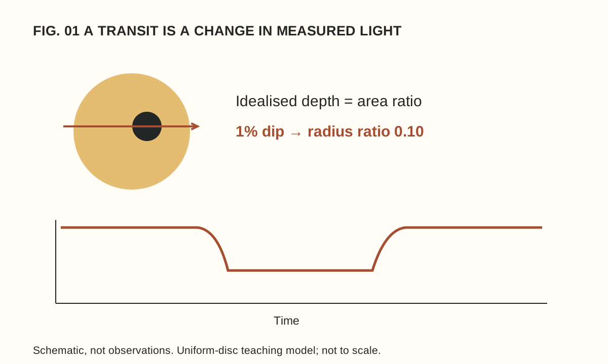
Schematic star and planet above a fictional light curve. A one-per-cent dip gives a radius ratio of 0.10 in the simplified uniform-disc model.

Many exoplanet discoveries begin with a star that becomes slightly dimmer. The planet itself may never appear as a resolved dot in the discovery data. Instead, astronomers measure how the light changes and ask which physical explanations can account for the pattern.

That makes a transit a good introduction to scientific inference. The observation is a series of brightness measurements. A planet’s size, orbit or atmosphere is a conclusion built from those measurements together with a model and other information. Keeping those layers separate makes the result more impressive, not less.

First, identify the observation

A transit occurs when a planet passes across its star from our line of sight. Some starlight is blocked, producing a dip. The alignment matters: a planet can orbit a star without crossing its visible disc from our viewpoint. ESA’s overview of detection methods explains why transits are only one route to finding worlds.

A light curve places time on one axis and measured brightness on the other. It is not a photograph of the planet’s path. A smooth illustrative curve can help explain the idea, but real observations contain scatter and may have gaps. Always read whether a figure contains measurements, a fitted model or an artist’s schematic.

The diagram accompanying this article is a schematic. Its scale and dip have been chosen for readability and do not represent a discovery. That label is part of the information: without it, a neat drawing can accidentally imply a precision that was never measured.

A deliberately simple size calculation

Imagine an evenly bright circular star and a much smaller opaque planet crossing fully in front of it. In this idealised model, the fraction of light blocked is approximately the planet’s disc area divided by the star’s disc area. ESA’s educational transit calculation develops this area-ratio relationship.

Suppose our fictional star has a normalised brightness of 1.000 outside transit and 0.990 at the flat part of the dip. The drop is 0.010, or one per cent. Because circle area depends on radius squared, the radius ratio is the square root of 0.010: 0.10.

The planet’s radius is therefore one tenth of the star’s radius in this model. Notice what we have not found: an absolute radius. If the star were twice as large, the same relative dip would correspond to a planet twice as large. Knowledge of the star is part of the planet measurement.

Now change the invented dip to 0.0025, or a quarter of one per cent. Its square root is 0.05. The inferred radius ratio is half the previous value, even though the blocked light is one quarter. This small calculation prevents a common mistake: interpreting a percentage loss of light as the same percentage of radius.

Why the real calculation is richer

A real star is not an evenly bright paper disc. Brightness varies across its face, and the path of the planet affects the shape of the dip. A grazing crossing requires different treatment from one in which the planet passes fully across the visible disc. Instrument behaviour and other light in the measurement also matter.

ESA’s Cheops explanation describes using the detailed transit shape, including its beginning and end, to characterise a system. Our square-root exercise captures the central geometry while intentionally leaving those additional effects out.

This is how an approximation should be used: state its assumptions, learn the relationship it reveals and avoid claiming that it replaces the full analysis. A simple model is valuable precisely because we know where it stops.

Repeated dips introduce another question

In an invented observation log, suppose similar dips occur at day 2, day 7 and day 12. The spacing suggests a five-day repetition. Before calling that the orbital period, ask whether observations were continuous, whether other dips could have been missed and whether the events have consistent shapes.

If the telescope observed only at certain intervals, the sampling pattern can affect what appears in the record. A convincing interpretation uses the full timing and uncertainty information, not three marks selected because they make a tidy pattern. The next predicted event is also an opportunity to test the explanation.

Not every dip establishes a planet. Other stellar configurations or instrumental effects can imitate parts of a transit signal. Follow-up observations are therefore an essential part of the story. A candidate is a question worth investigating, not a less exciting word that a headline should quietly remove.

Different measurements answer different questions

NASA’s guide to finding and characterising exoplanets contrasts transits with radial-velocity measurements, which examine shifts in starlight associated with motion along our line of sight. Combining suitable measurements can constrain properties that one method alone cannot establish.

Size is not the same as mass, and neither automatically supplies a detailed interior map. Even when a mean density can be estimated, different structures may be consistent with the available information. The useful reading habit is to ask what was measured directly and what range of models remains plausible.

Likewise, detecting a planet does not demonstrate habitability or life. Those are additional questions requiring additional evidence. A colourful illustration of oceans or clouds should be read as an illustration unless its caption specifies a different basis.

A three-line reading habit

When you next encounter an exoplanet story, write three short notes: observation, inference and uncertainty. For our fictional case they might read “a one-per-cent repeating dip”, “a radius ratio near one tenth under a simple model” and “stellar size, transit geometry and alternative explanations still matter”.

That habit transfers well beyond astronomy. Our guide to measurement uncertainty shows why a precise-looking number needs a description of how it was obtained. The remarkable achievement is not that a dip speaks for itself, but that careful observation and tested models can turn starlight into knowledge about a world we cannot directly see.