
Many exoplanet discoveries begin with a star that becomes slightly dimmer. The planet itself may never appear as a resolved dot in the discovery data. Instead, astronomers measure how the light changes and ask which physical explanations can account for the pattern.
That makes a transit a good introduction to scientific inference. The observation is a series of brightness measurements. A planet’s size, orbit or atmosphere is a conclusion built from those measurements together with a model and other information. Keeping those layers separate makes the result more impressive, not less.
First, identify the observation
A transit occurs when a planet passes across its star from our line of sight. Some starlight is blocked, producing a dip. The alignment matters: a planet can orbit a star without crossing its visible disc from our viewpoint. ESA’s overview of detection methods explains why transits are only one route to finding worlds.
A light curve places time on one axis and measured brightness on the other. It is not a photograph of the planet’s path. A smooth illustrative curve can help explain the idea, but real observations contain scatter and may have gaps. Always read whether a figure contains measurements, a fitted model or an artist’s schematic.
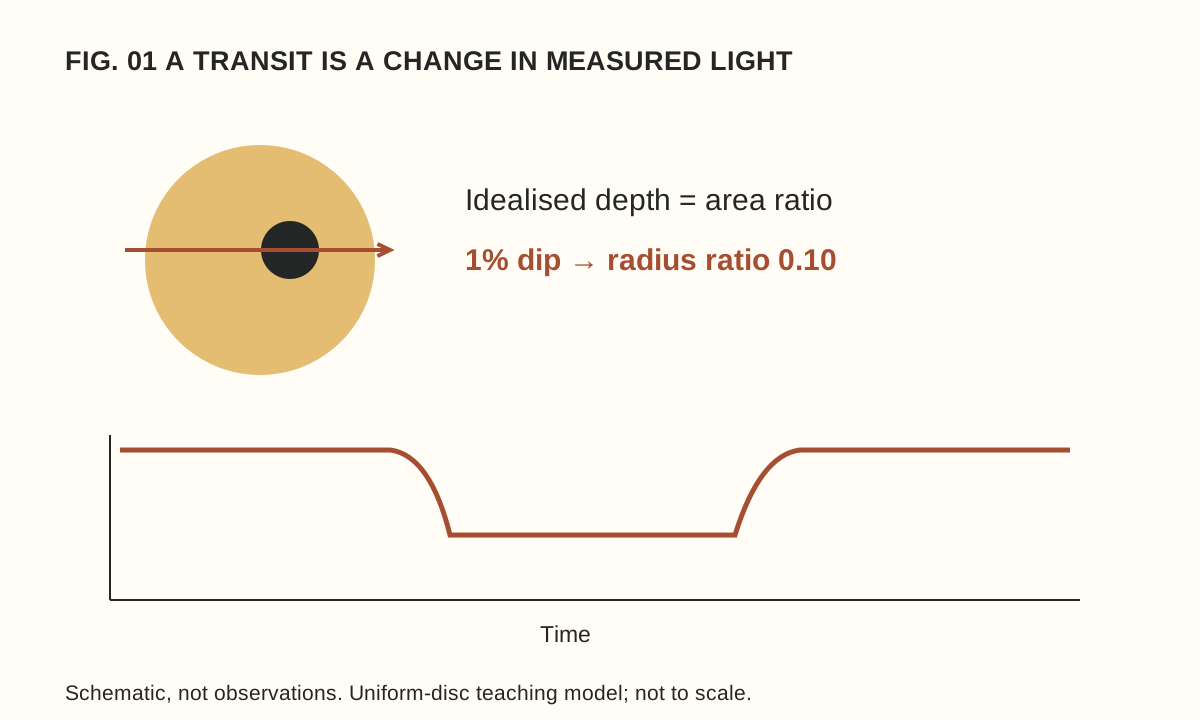
The diagram accompanying this article is a schematic. Its scale and dip have been chosen for readability and do not represent a discovery. That label is part of the information: without it, a neat drawing can accidentally imply a precision that was never measured.
A deliberately simple size calculation
Imagine an evenly bright circular star and a much smaller opaque planet crossing fully in front of it. In this idealised model, the fraction of light blocked is approximately the planet’s disc area divided by the star’s disc area. ESA’s educational transit calculation develops this area-ratio relationship.
Suppose our fictional star has a normalised brightness of 1.000 outside transit and 0.990 at the flat part of the dip. The drop is 0.010, or one per cent. Because circle area depends on radius squared, the radius ratio is the square root of 0.010: 0.10.
The planet’s radius is therefore one tenth of the star’s radius in this model. Notice what we have not found: an absolute radius. If the star were twice as large, the same relative dip would correspond to a planet twice as large. Knowledge of the star is part of the planet measurement.
Now change the invented dip to 0.0025, or a quarter of one per cent. Its square root is 0.05. The inferred radius ratio is half the previous value, even though the blocked light is one quarter. This small calculation prevents a common mistake: interpreting a percentage loss of light as the same percentage of radius.
Why the real calculation is richer
A real star is not an evenly bright paper disc. Brightness varies across its face, and the path of the planet affects the shape of the dip. A grazing crossing requires different treatment from one in which the planet passes fully across the visible disc. Instrument behaviour and other light in the measurement also matter.
ESA’s Cheops explanation describes using the detailed transit shape, including its beginning and end, to characterise a system. Our square-root exercise captures the central geometry while intentionally leaving those additional effects out.
This is how an approximation should be used: state its assumptions, learn the relationship it reveals and avoid claiming that it replaces the full analysis. A simple model is valuable precisely because we know where it stops.
Repeated dips introduce another question
In an invented observation log, suppose similar dips occur at day 2, day 7 and day 12. The spacing suggests a five-day repetition. Before calling that the orbital period, ask whether observations were continuous, whether other dips could have been missed and whether the events have consistent shapes.
If the telescope observed only at certain intervals, the sampling pattern can affect what appears in the record. A convincing interpretation uses the full timing and uncertainty information, not three marks selected because they make a tidy pattern. The next predicted event is also an opportunity to test the explanation.
Not every dip establishes a planet. Other stellar configurations or instrumental effects can imitate parts of a transit signal. Follow-up observations are therefore an essential part of the story. A candidate is a question worth investigating, not a less exciting word that a headline should quietly remove.
Different measurements answer different questions
NASA’s guide to finding and characterising exoplanets contrasts transits with radial-velocity measurements, which examine shifts in starlight associated with motion along our line of sight. Combining suitable measurements can constrain properties that one method alone cannot establish.
Size is not the same as mass, and neither automatically supplies a detailed interior map. Even when a mean density can be estimated, different structures may be consistent with the available information. The useful reading habit is to ask what was measured directly and what range of models remains plausible.
Likewise, detecting a planet does not demonstrate habitability or life. Those are additional questions requiring additional evidence. A colourful illustration of oceans or clouds should be read as an illustration unless its caption specifies a different basis.
A three-line reading habit
When you next encounter an exoplanet story, write three short notes: observation, inference and uncertainty. For our fictional case they might read “a one-per-cent repeating dip”, “a radius ratio near one tenth under a simple model” and “stellar size, transit geometry and alternative explanations still matter”.
That habit transfers well beyond astronomy. Our guide to measurement uncertainty shows why a precise-looking number needs a description of how it was obtained. The remarkable achievement is not that a dip speaks for itself, but that careful observation and tested models can turn starlight into knowledge about a world we cannot directly see.